Beschreibung zeitkontinuierlicher Systeme

Allgemein

Beschreibung

der Begriffe siehe Abschnitt sub:Systemstruktur-eines-Modells.

• Im Nachfolgenden werden Vektorpfeile der Einfachheit halber weggelassen.

Zustandsgleichung / Systemfunktion

$$\dot{x}\left(t\right) = \frac{dx\left(t\right)}{dt}$$

$$= \left(\begin{array}{c} \dot{x}_{1}\left(t\right)\\ \vdots\\ \dot{x}_{n}\left(t\right)\end{array}\right)$$

$$= \left(\begin{array}{c} f_{1}\left(x\left(t\right),u\left(t\right)... ...\vdots\\ f_{n}\left(x\left(t\right),u\left(t\right),t\right)\end{array}\right)$$

$$= f\left(x\left(t\right),u\left(t\right),t\right)$$

Ausgangsgleichung

$$y\left(t\right) = g\left(x\left(t\right),u\left(t\right),t\right)$$

$$= \left(\begin{array}{c} g_{1}\left(x\left(t\right),u\left(t\right)... ...\vdots\\ g_{m}\left(x\left(t\right),u\left(t\right),t\right)\end{array}\right)$$

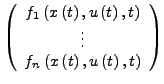
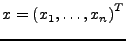
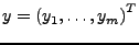
Zustandsgrößen

$x=\left(x_{1},\ldots,x_{n}\right)^{T}$

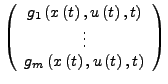
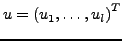
Stellgrößen

$u=\left(u_{1},\ldots,u_{l}\right)^{T}$

Ausgangsgrößen

$y=\left(y_{1},\ldots,y_{m}\right)^{T}$

Verschiedene Systemdynamiken

Höhere Ordnung

Jedes System von Differentialgleichungen höherer Ordnung kann auf ein System 1. Ordnung transformiert werden.
Hierzu wird bei einem System $k$-ter Ordnung 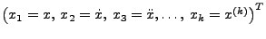$\left(x_{1}=x,\: x_{2}=\dot{x},\: x_{3}=\ddot{x},\ldots,\: x_{k}=x^{\left(k\right)}\right)^{T}$ als Systemzustandmit entsprechender Systemfunktion genommen.

autonomes System

Ein System das nicht explizit von $t$ abhängt wird als autonom bezeichnet.
Jedes System lässt sich durch Hinzunahme von $t$ zu den Systemzuständen mit $\dot{t}=1$ in ein autonomes System transformieren.

lineare Systemdynamik

hat folgende Gestalt

$$\dot{x} = f\left(x,u\right)=Ax+Bu$$

$$y = g\left(x,u\right)=Cx+Du$$

mit konstanten (oder rein zeitabhängigen) Koeffizientenmatrizen

$$A\in\mathbb{K}^{n\times n} B\in\mathbb{K}^{n\times l}$$

$$C\in\mathbb{K}^{m\times n} D\in\mathbb{K}^{m\times l}$$